Top-k and top-p sampling: how an LLM picks its next token

The interactive below shows both strategies side by side. Flip between top-k, top-p, and greedy, drag the cutoff slider, and switch between three preset prompts to see how the distribution's shape changes everything. The glowing columns above the bars show which tokens are actually getting drawn, accumulating in real time.

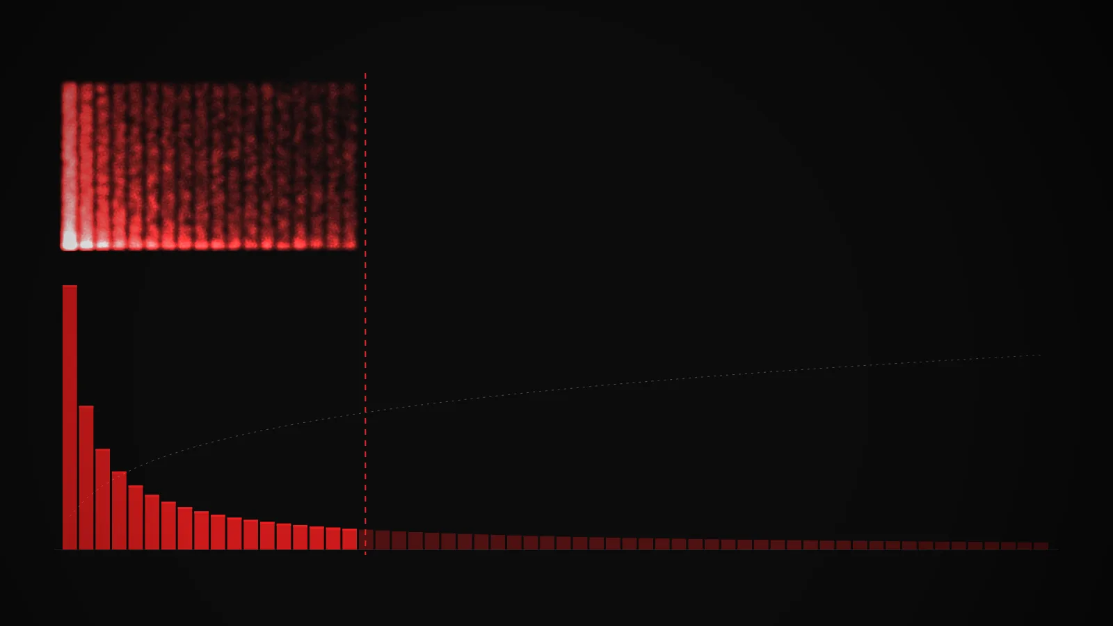
What you're seeing

The bars along the bottom are a language model's next-token probability distribution for a given prompt, sorted from most to least likely. Each bar is one candidate token . The tall ones on the left are the model's top guesses. The long flat tail on the right is everything it considers barely plausible.

The vertical red line is the cutoff. Bars to the left of it are the eligible set, the tokens that are actually allowed to be sampled. Bars to the right are dimmed, meaning the model cannot pick them no matter how the dice fall. The dashed line climbing over the bars is the cumulative probability (CDF), which is what top-p is looking at when it decides where to cut.

Above the histogram, every sample drawn drops a small red dot in a vertical column above the token it landed on. Over thousands of samples, the most-drawn tokens grow bright columns and the rarely-drawn ones stay dark. That column pattern is the actual output distribution of the sampler.

A few things to try in the demo:

• Pick the peaked prompt ("The capital of France is") and flip to greedy. Only one column grows. That is what deterministic decoding looks like.
• Switch to the flat prompt ("Once upon a") and drag K from 40 down to 5. Watch how many plausible tokens you just disqualified. A rank cutoff feels brutal on a flat distribution.
• Switch to top-p mode on the same flat prompt and drag P. The eligible set tracks the shape of the distribution instead of the position of the slider. That is the whole point.
• Hit reset and let N climb past 20,000. The column heights stabilize into the true renormalized probabilities of the eligible set. That is what the model's output distribution looks like after sampling.

How it actually works

A language model's final layer emits one raw score (a logit ) per token in its vocabulary, which softmax turns into a probability distribution over the whole vocab. Typical vocab sizes are in the tens of thousands. If the model just sampled directly from that raw distribution, it would occasionally pick genuinely terrible tokens from the long tail, and the output would feel unhinged. Top-k and top-p exist to cut the tail off.

Top-k sorts the tokens by probability, keeps the top K, zeroes out everything else, and renormalizes the kept probabilities so they sum to 1. The model then samples from that renormalized distribution. K is a fixed number, usually something like 40 or 50 in practice.

Top-p (also called nucleus sampling) works in descending probability order: it adds tokens to the eligible set one at a time until the running total of their probabilities crosses a threshold P, then stops. Everything past that point is discarded, the kept set is renormalized, and the model samples. P is usually 0.9 or 0.95.

The difference matters when the distribution's shape changes. On a peaked distribution where one token has most of the mass, top-p will keep almost nothing past that one token. On a flat distribution where probability is spread across many tokens, top-p will keep many of them. Top-k keeps the same number either way, which is its core weakness.

Greedy decoding is the degenerate case: always pick the argmax, sample nothing. It is deterministic and occasionally useful (code generation, structured output), but on longer text it tends to fall into repetitive loops because small probability differences compound over many steps.

One more piece: temperature scales the logits before the softmax, which flattens or sharpens the distribution. Order matters. Apply top-p after temperature scaling and the same p value produces a very different eligible set: tight at low temperature, loose at high. Most production stacks apply temperature first, then top-k or top-p. A few apply them in the other order and get noticeably different behavior.

Both strategies can combine. Some stacks do top-k first to cap the size of the eligible set, then top-p inside that, then sample. The exact pipeline varies by framework, which is one reason two implementations of "the same" sampler can produce different text for the same prompt and seed.

Picking the right values

There is no universal "correct" setting. The right cutoff depends on what you want the output to be.

• Code and structured output: use greedy or a very low temperature with a small k (1 to 5) or a low p (0.1 to 0.3). You want the best single guess, not creativity.
• Conversational or factual answers: temperature around 0.7 and top-p around 0.9 is a common default. Enough variance to sound natural without letting obviously wrong tokens slip in.
• Creative writing or brainstorming: higher temperature (1.0 to 1.3) with top-p at 0.92 to 0.95 opens the tail without descending into nonsense.

A common mistake is treating these values as universal. A top-p of 0.9 that works for storytelling will not be what you want for generating SQL. Tune per task, and test at a few different settings before committing to a default.

To go deeper on the upstream model mechanics, the gradient descent demo shows how models get trained in the first place. For the full vocabulary of inference terms, see the glossary.

Key takeaways

• Top-k is shape-blind. The same k of 40 behaves almost-greedy on a peaked distribution and almost-random on a flat one, because a rank cutoff ignores what the probabilities actually look like.
• Top-p is shape-aware. The eligible set grows when the model is unsure and shrinks when it is confident, because the cutoff is based on cumulative probability mass, not rank position.
• The cutoff only decides which tokens are on the ballot. The actual next token is still sampled at random from the renormalized probabilities inside the eligible set, not picked by a rule.
• Temperature reshapes the distribution before the cutoff is applied. Top-p at a low temperature produces a much tighter eligible set than top-p at a high temperature, even with the same p value.