Continuous batching: why your API latency varies

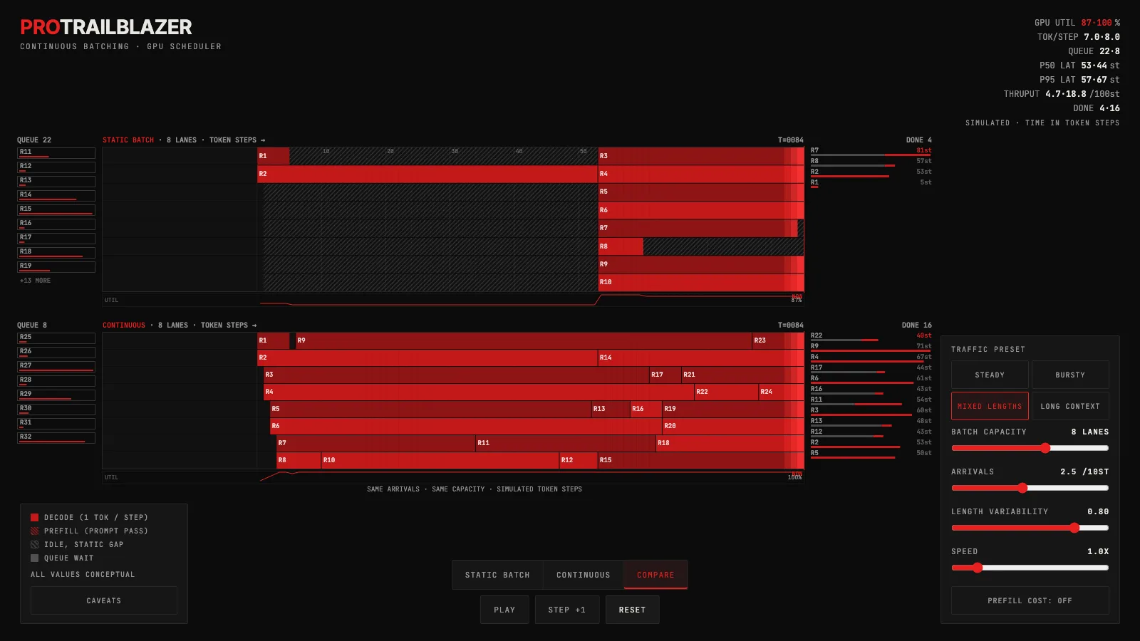
The interactive below runs two schedulers on the same seeded request stream. Switch between Static Batch, Continuous, and Compare modes, adjust the traffic preset and batch capacity, and step through one iteration at a time to see exactly when a lane goes idle and when it gets refilled.

What you're seeing

The scene is a Gantt-style scheduler timeline. On the left, a queue column shows requests waiting to be assigned a lane. In the center, each horizontal lane is one slot in the batch. Each cell in a lane is one token step: solid red means the lane is decoding (producing one token per step), hatched dark red marks the prefill pass (processing the prompt before the first output token appears), and striped gray marks idle static-batch dead capacity. Completed requests stack at the right with a latency bar broken into wait, prefill, and decode time. The HUD shows GPU utilization, tokens per step, queue depth, p50 and p95 latency in token steps, throughput per 100 steps, and total completed requests.

In Compare mode, both panes run on one clock so the gap between schedulers accumulates in real time. The queue drains at different rates, the utilization sparklines diverge, and the latency percentiles in the HUD update side by side so you can read the exact delta between strategies.

All values are labeled SIMULATED. Time is measured in token steps, not milliseconds. The simulation uses a deterministic seed (1337) so Reset and preset changes replay the same trace for the same settings.

A few things to try:

• Start in Compare mode with the Mixed Lengths preset. Watch the striped idle gaps accumulate in the static pane while the continuous pane keeps lanes filled. The p95 latency numbers in the HUD drift apart within a few dozen steps.
• Slide length variability to zero with Steady traffic. When every request decodes the same number of steps, every lane finishes at the same time, no lane strands early, and the two schedulers behave nearly identically. The utilization gap nearly closes.
• Push the arrival rate above what the lanes can handle. The queue column grows in both panes under overload. Continuous drains it faster but does not repeal queueing. This is the clearest signal that batching strategy and capacity are separate levers.
• Enable Prefill cost and switch to Long Context. Long prompts charge several steps of hatched prefill before decode starts, delaying the first output token and slowing the lanes around them. You can see why long-context requests raise p95 latency more than p50.
• Use Step +1 while paused. Each click advances one scheduler iteration. In the continuous pane, you can catch the exact step where a finished lane refills from the queue. In the static pane, that slot stays gray until the rest of the batch finishes.

How continuous batching actually works

LLM generation is iterative. Each forward pass produces one output token per active lane and returns control to the scheduler. That natural decision point is what makes continuous batching possible: after every iteration, the scheduler checks whether any lane finished and, if so, immediately pulls the next request from the queue into that slot.

Static batching does not check between iterations. The scheduler assembles a batch, runs it until the longest request in the batch finishes, and only then accepts the next group. If one request decodes 8 steps and another decodes 40, the 8-step lane sits dark for the remaining 32 steps while the batch holds its size.

The mechanism that makes this affordable is the KV cache. Each request stores its attention keys and values for every position generated so far. When a new request joins mid-batch, it computes its own KV entries from scratch during prefill, then runs in parallel with the requests already decoding. Memory for the KV cache grows with the number of active requests and their sequence lengths, which is why real serving systems add KV cache memory management and paging on top of the basic continuous-batching logic.

Prefill and decode are distinct phases. During prefill, the server processes the entire prompt in a single (or a few) forward passes before the first output token appears. During decode, the model generates one token per step per lane. Long prompts can occupy a lane for many prefill steps, which is why the simulation separates the two visually and why real systems sometimes schedule prefill and decode on separate resources.

Why utilization is not the whole story

Continuous batching raises GPU utilization, but utilization is not the metric users experience. What users feel is time-to-first-token (TTFT) and inter-token latency. A fully utilized GPU can still have high TTFT if the queue is long and each incoming request has to wait for a lane to open.

The context window length of each request determines how much KV cache memory it needs and for how long. A server running 8 lanes at a long context window may be as memory-constrained as one running 32 lanes at a shorter window. Real serving systems use admission control to refuse requests that would overflow KV cache memory, which is a limit the simulation's caveats panel calls out explicitly.

The p50 latency the demo shows is the median total request latency in token steps. The p95 is the 95th percentile. In traffic with uniform decode lengths, the two track closely. Add length variability and the p95 climbs because a small fraction of long requests block lanes and delay the queue behind them. Continuous batching reduces that effect but does not eliminate it, because the long requests are still consuming a lane for their full decode length.

To see how each output token is produced step by step, the autoregressive generation walkthrough covers the full path from prompt through the KV cache to a sampled token. For the tradeoff between compute per step and output quality, see inference-time compute.

Frequently asked questions

Key takeaways

• Static batching's real cost is variance, not batching. Every request in the batch holds its lane until the longest one finishes, so a lane that finishes early sits as dead capacity and a short request inherits the latency of its slowest batchmate.
• Continuous batching only works because LLM generation is iterative. One token per lane per step gives the scheduler a decision point at every iteration, so a freed lane can be refilled between tokens instead of between batches.
• When decode lengths are uniform, the two schedulers behave almost the same. Load the steady preset and slide length variability to zero and the gap in utilization and p95 nearly closes, because no lane ever finishes far ahead of its batch.
• Continuous batching raises utilization, it does not repeal queueing. Push the arrival rate past what the lanes can decode and the queue grows in both panes; the continuous pane just drains it faster.
• Prefill and decode are separate costs. A long prompt occupies a lane for several steps before its first output token appears, which is part of why long-context requests slow down the requests around them.