Inference-time compute: more samples, smarter answers

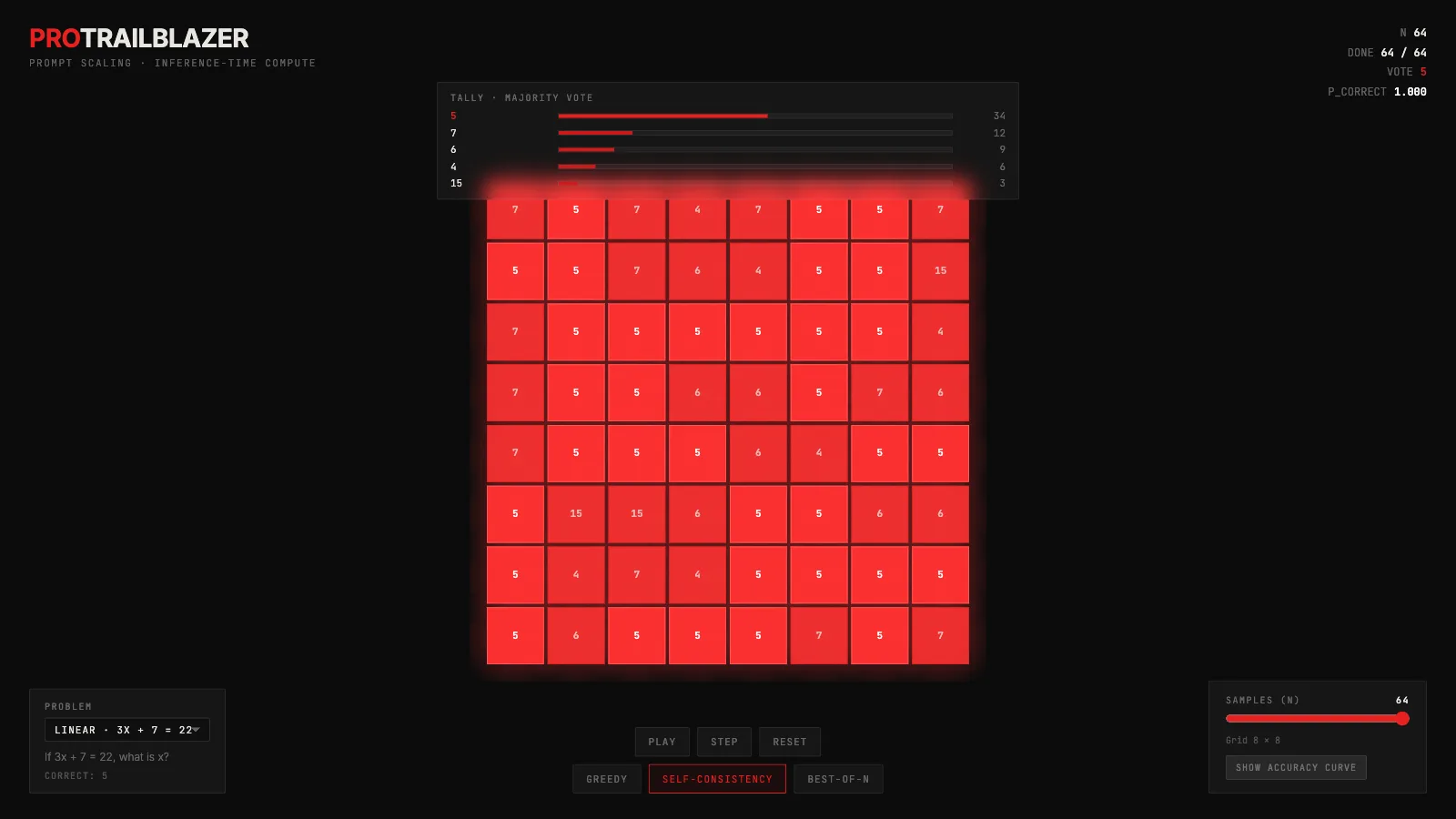
The interactive below shows inference-time compute at work. Each cell is one independent reasoning chain solving the same problem. Drag the samples slider from 1 to 64, switch between three strategies, pick a harder problem, and toggle the accuracy curve. The thing to watch: the weights never change. Only the amount of compute spent at question time does, and the accuracy climbs anyway.

What you're seeing

A grid of small red cells, each one an independent reasoning chain attacking the same question. Darker cells are idle or thinking. The brief flash and bloom is the moment a chain commits to a final answer. Cells that agree with the majority stay bright red. Cells that voted for a minority answer dim to a duller red, marking them as outliers.

Each cell shows its current reasoning step as a tiny monospace string. For the linear equation problem you will see things like 3x=15 tick through to =5. For the prime-check problem you will see divisors being tried one at a time. These steps are the cell's internal thinking made legible. Every chain is following its own sampled trajectory, not the same path.

The tally panel above the grid collects the votes. Each distinct answer gets a bar proportional to its share of committed chains. The leading answer lights up bright red and the whole panel flashes when a new commit flips the leader. The stats row in the top-right keeps the running count: N is the current sample budget, DONE is the chains that have committed, VOTE is the current majority answer, P_CORRECT is the probability that this majority is correct at this N.

A few things to try in the demo:

• Set samples to 1 and run the train catch-up problem ten times. Most runs will land on a wrong answer like 4:26 PM or 8:00 PM. A single sample is a coin flip weighted by whatever the most likely wrong paths happen to be.
• Drag samples to 32 on the same problem. The tally stabilizes on 7:00 PM within a few commits. The correct trajectory is not the plurality on its own, but it is the most agreed-upon answer across the distinct wrong paths.
• Switch to GREEDY and drag the slider. Nothing changes. Every cell runs the same deterministic trajectory, so P_CORRECT is flat regardless of N. This is the baseline that inference-time compute improves on.
• Turn on the accuracy curve overlay. It plots P_CORRECT across 200 silent trials at N of 1, 2, 4, 8, 16, 32, 64. The shape is the real sub-logarithmic scaling curve from the self-consistency literature, just derived from a hand-authored distribution instead of a live model.

How it actually works

Every language model is a probability distribution over next- tokens . Sample from that distribution and you get one answer. Sample again and you get a different answer, because the middle of any nontrivial reasoning path has real uncertainty in it. A chain-of-thought that spells out the intermediate steps before the final answer exposes that uncertainty instead of hiding it. Inference-time compute leans on exactly that property: instead of asking the model once, ask it many times and treat the population of answers as the signal.

Three common strategies for turning many samples into one answer:

• Greedy decoding. At every step, take the single most likely token. One deterministic trajectory, one deterministic answer. See greedy decoding for the full picture. Sampling more than one chain buys you nothing here because every chain is identical.
• Self-consistency . Sample N independent chains at a nonzero temperature , extract each chain's final answer, apply majority voting to return the most common one. This is the standard setup from the self-consistency paper, and it is what the demo's default strategy does.
• Best-of-N . Sample N independent chains, score each one (by a reward model, a verifier, or the model's own log-probability on the answer), then keep the highest-scoring chain's answer. This replaces voting with picking, which works well when your scoring function is trustworthy and badly when it is not.

Why does voting work? Because the model's error is not uniform. On a non-trivial question, there is usually one correct answer and many distinct wrong ones. A single chain might slip in any of a dozen ways, but slipping the exact same way twice requires two chains to make the exact same mistake. As N grows, correct answers accumulate on one bucket while wrong answers smear across many. The majority bucket wins even if it has less than half the single-sample mass, as long as it beats each wrong bucket individually.

N is a hyperparameter you set per request. It trades wall-clock and dollars for accuracy. Scaling from N=1 to N=8 is usually a big jump. From N=8 to N=32 is a smaller one. From N=32 to N=64 is often negligible. The accuracy curve flattens out because you hit a floor set by how often the correct trajectory is even in the sample at all. Once you are reliably including the right answer somewhere, more samples do not help.

The o1, o3, and R1 family of reasoning models take this idea one step further. Instead of just drawing N parallel samples, they are trained to generate very long chains of reasoning within a single response, and to use learned value heads to decide which internal branches to expand. The scaling axis is the same though: spend more compute at inference time, get better answers, without changing the weights.

When this stops working

Three failure modes to keep in mind.

The first is when the model is systematically wrong. If the most likely wrong answer has more mass than the correct one and every other wrong answer combined, majority vote converges to the wrong answer, faster as N grows. More compute makes a confidently wrong model more confidently wrong.

The second is open-ended generation. Majority voting needs a discrete answer to tally. For tasks like essay writing or code generation, there is no single correct string to vote on, so self-consistency does not apply directly. Best-of-N with a good scoring function works instead, but now everything rides on whether the scoring function is actually calibrated.

The third is cost. At N=32 you are paying 32x the tokens you would for a single response. For low-stakes chat this is absurd. For high-stakes reasoning (math, code, medical, legal, trading) it can still be the cheapest way to buy accuracy, because the alternative is training a bigger model and that bill is much higher.

For adjacent sampling concepts see the temperature post and the top-k and top-p post. For the broader vocabulary around inference, see the glossary.

Key takeaways

• Self-consistency works because wrong answers disagree with each other while correct answers tend to agree. The signal concentrates on a single number while the noise spreads across many.
• The accuracy-vs-N curve is sub-logarithmic. Most of the gain is between N=1 and N=8. Doubling to N=64 usually buys you a few more percentage points at 8x the cost.
• Best-of-N only beats majority vote when your scoring function is trustworthy. If the model is confidently wrong, best-of-N amplifies the wrong answer instead of averaging it out.
• Greedy decoding caps accuracy at whatever a single deterministic trajectory gives you. Adding compute to a greedy chain does nothing, because there is no sampling variance to average over.
• This is why the new reasoning models feel smarter without being larger. They spend more compute at inference time, not during training. The weights are the same. The wall-clock is not.