HNSW vector search: how a layered graph finds neighbors fast

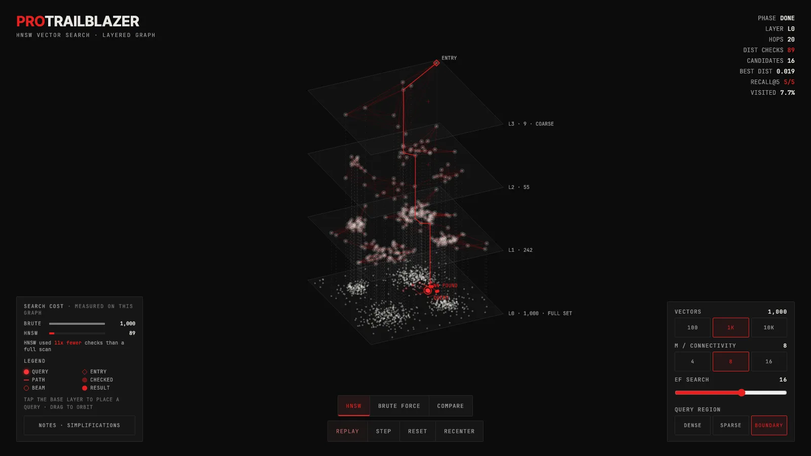
The interactive below builds a real HNSW index in your browser from seeded 2D points and runs a genuine graph traversal on it. Pick a dataset size, adjust M and efSearch, and either tap the base layer to place your own query or pick one of the presets. You can race HNSW against brute force in compare mode, step through one hop at a time, or orbit the isometric stack to see how the layers relate.

New tab

Demo

HNSW vector search: a layered graph, hop by hop

A real HNSW index built in the page: watch the search hop a four-layer graph from coarse to fine, then race it against a brute-force scan and tune efSearch and M.

Built with Canvas 2D. The index is built and searched locally in the page: hops, distance checks, recall@5, and visited share are measured on the rendered graph, not simulated.

What you're seeing

The canvas renders an isometric stack of four graph layers, labeled L0 through L3. L0 at the base holds every vector point. L1, L2, and L3 above it are progressively sparser random samples of those same points, connected by longer-range edges. The search enters at the top layer and descends, greedy-hopping toward the query on each layer before dropping to the one below. On the base layer it switches to a beam search, keeping the efSearch best candidates in a priority queue until no closer node can be found.

The HUD in the top-right tracks everything as it happens: current layer, total graph hops, distance checks so far, number of beam candidates, best distance found, recall@5 versus a brute-force scan of the same graph, and the share of all vectors visited. Distance checks and visited share are measured on the rendered graph, not simulated, so the numbers reflect the index actually built in the page.

In compare mode, two searches race side by side: the HNSW path in red and a brute-force sweep shown in white. The left panel's progress bars fill at their own pace so you can watch the check counts diverge. At 10K vectors the gap is dramatic.

A few things to try:

Jump from 100 to 10K vectors and watch the visited share. Brute force always checks every stored vector, so its bar fills at the same rate regardless of size. The HNSW visited share shrinks as the dataset grows because the upper layers span more ground per hop.
Drag efSearch down to 2 and then back up to 64. Recall@5 responds: at low efSearch you may see 3/5 or 4/5 rather than 5/5. This is the core tradeoff, not a bug. When recall drops below what the application needs, raise efSearch at serve time.
Switch M from 4 to 16 and rebuild. Higher M means more connections per node on every layer, so the beam has more routes to explore. Distance checks typically rise, but recall tends to hold at lower efSearch values. M is a build-time decision, unlike efSearch.
Tap the BOUNDARY query preset. Edge queries are harder because the true neighbors cluster in one direction. Watch whether the greedy descent from upper layers enters the right neighborhood before the base-layer beam begins.
Use the step button to advance one hop at a time. You can follow each layer transition and see exactly when the search commits to a neighborhood. The top-layer hop count is usually very small (one to three) before the algorithm descends.

How HNSW actually works

A vector database stores as high-dimensional points and answers nearest-neighbor queries over them. The naive approach measures the distance from the query to every stored point and returns the closest ones. That is exact, but it costs one distance check per stored vector on every query. At tens of millions of vectors the latency is unacceptable.

HNSW avoids the full scan by building a hierarchy of navigable graphs during index construction. Every vector is assigned to a level: all vectors live on L0, but a random fraction (controlled by a level multiplier) also appear on L1, a smaller fraction on L2, and so on. On each level, each node is connected to its M nearest neighbors among the nodes that share that level. The resulting graph has small-world properties: a few long-range shortcuts at the top and dense local connections at the base.

At query time, the search enters at the highest non-empty layer at a fixed entry point. It greedily hops to whichever neighbor is closest to the query until no neighbor is closer than the current node, then descends one level and repeats, starting from the landing node. On the base layer (L0) it switches from pure greedy to a beam search: it keeps an ordered list of the efSearch best candidates seen so far and continues expanding the closest unvisited one until the list stops improving. The result is the ef closest nodes found on L0.

The demo's construction is a teaching simplification. Each node is connected to its M kNN neighbors per layer rather than using the insert-one-at-a-time pruning heuristic that real HNSW implementations use. The demo also caps the graph at 4 layers for visual legibility. These differences are disclosed in the NOTES panel. The search itself is a genuine greedy-beam traversal on the graph actually built in the page.

What efSearch and M actually control

M is the graph's connectivity, baked in at index build time. It controls how many neighbors each node stores on each layer. Low M means sparse connections and fast hops but higher risk of the search entering a dead-end neighborhood and missing a true near neighbor. High M means more routes, better recall, and more memory per node. You cannot change M without rebuilding the index from scratch.

efSearch is the beam width on the base layer, and you can tune it per query at serve time without touching the index. A higher efSearch keeps more candidates in the priority queue at once, so the beam explores more of the local neighborhood before committing to a result. The tradeoff is latency: each additional candidate means additional distance checks. This is why operators typically build with a moderate M and adjust efSearch dynamically when downstream accuracy requirements change.

The recall@5 number in the HUD compares the 5 results HNSW returned to the 5 true nearest neighbors from a full scan. A score of 4/5 means one true neighbor was missed. That is the contract of an approximate index: you trade a small miss probability for skipping most of the distance checks. When you need guaranteed exact results, brute force (or exact indexes like flat FAISS) is the right tool, but at the scale where vector search matters, approximate is almost always the right default.

For a broader view of how retrieval fits into an LLM pipeline, the retrieval-augmented generation explainer walks through how nearest-neighbor search connects a query to a knowledge base before generation. And if you want to understand what goes into the vectors being searched, embeddings in 3D shows how semantic similarity maps onto geometric distance.

Frequently asked questions

Why is HNSW approximate instead of exact?

The greedy descent from upper layers commits to a neighborhood early. If the entry point on a layer happens to be far from the query's true neighborhood, the beam may converge on a local cluster that misses one or two true neighbors. Raising efSearch reduces this risk by keeping more candidates alive on the base layer, but it never eliminates it entirely without degenerating into a full scan. The approximation is the whole point: the algorithm is fast precisely because it stops exploring before it checks everything.

What is recall@5 and why does the demo track it?

Recall@5 is the fraction of the true 5 nearest neighbors that appear in the 5 results HNSW returned. A score of 5/5 means HNSW found every true neighbor; 4/5 means one was missed. The demo computes this live by running a full brute-force scan in the background and comparing the result sets. In production systems, recall@K at a target latency is the primary metric for tuning efSearch and M.

How does M affect index quality versus cost?

Higher M gives each node more neighbors on each layer, which means more paths through the graph and higher recall at the same efSearch, but memory per node grows linearly with M. A common production default is M=16 on the base layer and M=8 on upper layers (some implementations use 2M on L0). The right M depends on your dataset's intrinsic dimensionality and how much memory you can spare.

Why do the upper layers hold fewer points?

Each vector is assigned a maximum level during construction by drawing from a negative-exponential distribution. Most vectors land on L0 only; a fraction make it to L1; fewer still to L2; and so on. This exponential thinning is what gives HNSW its small-world topology: the sparse top layers span large distances quickly, and the dense base layer provides fine resolution. Without the thinning, all layers would be equally dense and the speed advantage would vanish.

Can HNSW handle filtered search or deletes?

The demo does not cover either, and they are genuinely hard problems. Deletes typically require a tombstone plus periodic re-indexing or a specialized soft-delete mechanism; true node removal risks disconnecting the graph. Filtered search (return neighbors that also satisfy a metadata predicate) can cause recall to collapse if the filter eliminates most candidates from the beam. Production systems handle this with pre-filtering, post-filtering, or hybrid indexes, each with its own recall tradeoffs.

Key takeaways

HNSW is approximate on purpose. A recall@5 below 5/5 is not a failure, it is the contract: you trade a small chance of missing a true neighbor for skipping almost all of the distance checks, and you buy recall back with efSearch when you need it.
efSearch and M are different kinds of knobs. efSearch is a per-query setting you can raise at serve time, while M is baked in when the graph is built, so fixing recall in production usually means turning up efSearch, not rebuilding the index.
The upper layers hold no extra information. Every vector lives on the base layer, and the layers above are just sparse random samples of the same points, acting as long-range shortcuts that get the search near the right neighborhood in a few hops.
The payoff scales with the dataset. Brute force pays one distance check per stored vector on every query, while HNSW's path barely grows, which is why the demo's visited share collapses when you jump from 100 to 10,000 vectors.